
Introduction of Downsampling
09/17/2019 Tags: Singal_ProcessAbstract
The sampling process is creating a discrete signal from a continuous process. And there are two common sampling processes: down-sampling and un-sampling. To put it simply, downsampling reduces the sample rate and upsampling increases the sample rate. In this post, I only recored the basic concepts of downsampling and the relevant information.
Dowmsampling
The idea of downsampling is removing samples from the time-domain signal.
The mathematical representation
Consider downsampling a discrete-time signal \(x_d[n]\) of length \(N\):
\[x_d[n] = x[nM]\]It means an integral multiplication increases the sample period of a discrete-time siganl by an integer \(M\). The replication period in the frequency domain is reduced by the same multiple.
The downsampling and spectral on continuous-time and discrete-time signal
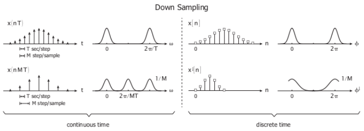
Note: Because downsampling by \(M\) may causes aliasing, the input signal should need the low-pass filter to prevent this aliasing.
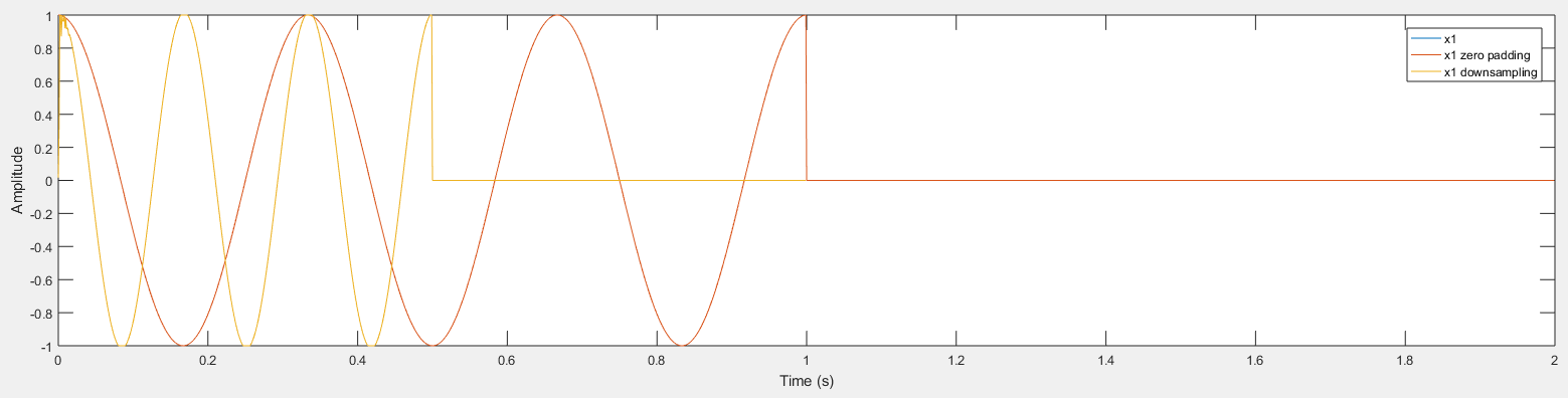
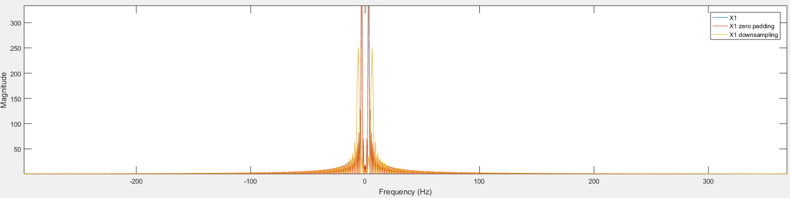
Example. Comparison of orignal signal, signal with zero padding and signal after downsampling
downsampling.m
% Sampling rate
fs = 1000;
% time duration (0 ~ 1 sec)
t = 0 : 1/fs : 1 - 1/fs;
% central frequency
f1 = 3;
fir_len = 31;

x1 = cos(2*pi*f1*t);

% FFT Without Zero-padding
L1 = length(x1);
X1 = fft(x1);

% FFT With Zero-padding
x1_zero = [x1 zeros(1, 1000)];
X1_zero = fft(x1_zero);
L1_zero = length(x1_zero);
t_zeropad = [0:L1_zero-1]/fs;

% FFT With downsampling
zero_padd = zeros(1, fir_len)'; % Zero-padding

% Downsampling
[x1_dwn] = downsample(x1', zero_padd);
x1_dwn = [x1_dwn ; zeros(1, 500)'];
X1_dwn = fft(x1_dwn);
L1_dwn = length(x1_dwn);
t_dwn = [0:L1_dwn-1]/fs;

% Plot
figure(1);
subplot(2, 1, 1);
plot(t, x1)
hold on
plot(t_zeropad, x1_zero)
hold on
plot(t_dwn, x1_dwn)
legend('x1','x1 zero padding', 'x1 downsampling')
xlabel('Time (s)')
ylabel('Amplitude')

subplot(2, 1, 2);
plot([-L1/2 : (L1/2 -1)]*fs/L1, fftshift(abs(X1)))
hold on
plot([-L1_zero/2 : (L1_zero/2 -1)]*fs/L1_zero, fftshift(abs(X1_zero)))
hold on
plot([-L1_dwn/2 : (L1_dwn/2 -1)]*fs/L1_dwn, fftshift(abs(X1_dwn)))
legend('X1','X1 zero padding', 'X1 downsampling')
xlabel('Frequency (Hz)')
ylabel('Magnitude')
Result: (Amplitude)
Result: (Frequency response)
Low-Pass Filter
A low pass filter is a filter which passes low-frequency signals and blocks high-freqnency signals.
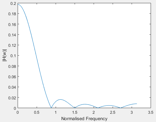
Example: Synthesising Finite Impulse Response Low-pass filter
In this example, the length of FIR low-pass filter is 32 and the sample rate is 512. And using frequency response of digital filter to calculate the fs-point frequency response vector \(h\) and the corresponding angular frequency vector \(w\) for the digital filter with transfer function coefficients stored in B and A.
lowpassFilter.m
% Sample rate
fs = 512;

% define the frequency response
f = linspace(0,1,32);

% from DC to fs/2
amp = [ 36339434    186540122  \
        477337738   760148204  \
        761699191   367623940  \
       -161062544  -385457455  ...
       -161535628   183023159  \
        237311199  -6177817    \
       -192162144  -96102896   \
        106831101   130670761  ...
       -24618760   -118427546  \
       -34616798    81016457   \
        65169473   -36314160   \
       -69585740    -2966005   ...
        54658857    29242864   \
       -28558676   -39001835   \
       -1087164     30114286   \
        27060106    9247146] / 2^31;

% Least-square linear-phase 10th order FIR filter design
B = firls(10, f, amp); % generate the coefficients
A = [1];
[h,w] = freqz(B, A, fs); % extract the transfer function from DC to fs/2

%Plot
plot(w, abs(h));
xlabel('Normalised Frequency')
ylabel('|H(w)|')
Result:
Zero-padding
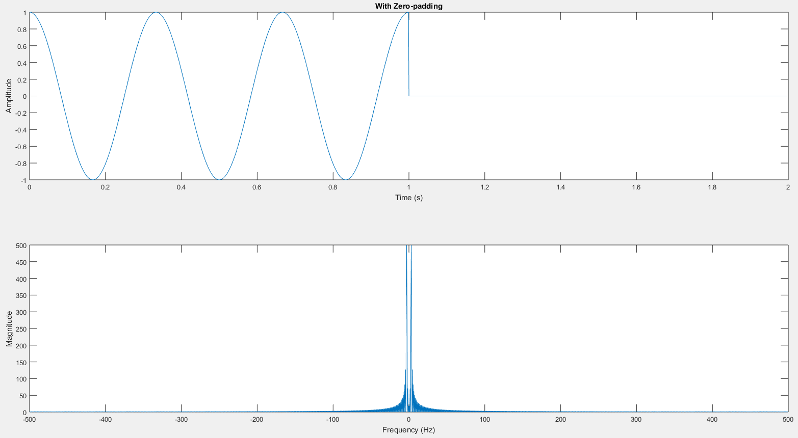
The zero-padding means changing the DFT-lenght \(N\) without adding more signal(i.e., information), which just results on a denser sampling of the underlying DTFT of the signal. To put it simply, the visible sampling on a denser frequency grid is achieved by zero-padding.
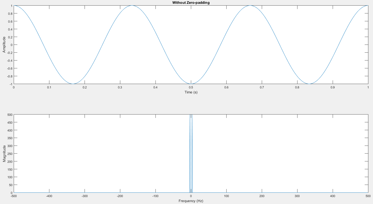
Example: FFT without zero-padding
fft.m
% Sample rate
fs = 1000;
% time duration (0 ~ 1 sec)
t = 0 : 1/fs : 1 - 1/fs;
% central frequency
f1 = 3;

x1 = cos(2*pi*f1*t);
L1 = length(x1);

% FFT Without Zero-padding
X1 = fft(x1);

% Plot
figure(1);
subplot(2, 1, 1);
plot(t, x1)
title('Without Zero-padding')
xlabel('Time (s)')
ylabel('Amplitude')
subplot(2, 1, 2);
plot([-L1/2 : (L1/2 -1)]*fs/L1, fftshift(abs(X1)))
xlabel('Frequency (Hz)')
ylabel('Magnitude')
Result:
Example: FFT with zero-padding
fftZeroPadding.m
% Sample rate
fs = 1000;
% time duration (0 ~ 1 sec)
t = 0 : 1/fs : 1 - 1/fs;
% central frequency
f1 = 3;

x1 = cos(2*pi*f1*t);

% FFT With Zero-padding
x1 = [x1 zeros(1, 1000)];
X1 = fft(x1);
L1 = length(x1);
t_zeropad = [0:L1-1]/fs;

% Plot
figure(2);
subplot(2, 1, 1);
plot(t_zeropad, x1)
title('With Zero-padding')
xlabel('Time (s)')
ylabel('Amplitude')
subplot(2, 1, 2);
plot([-L1/2 : (L1/2 -1)]*fs/L1, fftshift(abs(X1)))
xlabel('Frequency (Hz)')
ylabel('Magnitude')
Result:
Convolution in matlab
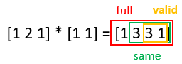
Syntax
w = conv(u,v,shape), where the shape is specified as ‘full’| ‘same’ | ‘valid’.
Example: The result of full convolution
\[\left[ 1 2 1 \right] * \left[ 1 1 \right] =\left[ 1 3 3 1 \right]\]Example: The result of same convolution
\[\left[ 1 2 1 \right] * \left[ 1 1 \right] = \left[ 3 3 1 \right]\]Example: The result of valid convolution
\[\left[ 1 2 1 \right] * \left[ 1 1 \right] = \left[ 3 3 \right]\]The diagrammatic convolution in matlab:
=========== To be continued…. ==========
Reference
[1] How Do I Upsample and Downsample My Data?
[2] Low-Pass Filtering by FFT Convolution
Feel free to leave the comments below or email to me. Any pieces of advice are always welcome. :)